Why are French Trains Late?
I have not been able to write for a while as the semester just started, but quite frankly that is a not an issue since no one other than me reads these posts :). Anyways, I wanted to do this week’s tidy tuesday as it was about French train delays which I got to get accustomated to while living in France.
library(tidyverse)
library(dynlm)
library(gganimate)
library(maptools)
library(maps)
library(lettercase)
library(magrittr)
library(ggfortify)
library(pander)
library(patchwork)
library(kableExtra)
trains_raw <- readr::read_csv("https://raw.githubusercontent.com/rfordatascience/tidytuesday/master/data/2019/2019-02-26/full_trains.csv")
trains_raw[4:5] %<>% mutate_all(funs(tolower)) %<>% mutate_all(funs(str_title_case))
trains_raw <- trains_raw[,- which(names(trains_raw) %in% c("comment_delays_on_arrival","comment_cancellations", "comment_delays_at_departure","delay_cause_external_cause", "delay_cause_rail_infrastructure", "delay_cause_traffic_management", "delay_cause_rolling_stock","delay_cause_station_management", "delay_cause_travelers"))]
trains <- trains_raw[complete.cases(trains_raw),]
small_trains <- readr::read_csv("https://raw.githubusercontent.com/rfordatascience/tidytuesday/master/data/2019/2019-02-26/small_trains.csv")
france <- map_data("france")Data Exploration
Let’s start by exploring the data. I could not find a really good model to predict the delay of trains on a station at a particular time, so I opted to build 3 models that predict the number of trains late by at least 15mins, 30mins, and 60 mins.
I used a stepwise regression to select variables but here are a few pretty plots to justify the selection of the variables.
The plots above are very interesting as they show a clear relationship where the variance increases as the x-values increase. This makes poisson regression a good choice to have a better fit as x-values increase. I did however use a linear regression for trains that were late by at least 15 mins as the fit was better when looking at the AIC and \(R^2\).
g1 <-
    ggplot(data = trains) + geom_point(aes(x = total_num_trips, y = num_greater_15_min_late)) + geom_smooth(
    aes(x = total_num_trips, y = num_greater_15_min_late),
    method = "lm",
    formula = y ~ poly(x, 2)
    ) + xlab("Total number of trains in the time period") + ylab("Number of trains greater than 15 min late") + labs(title = "Linear Regression for Trains that are Later than 10 min") + theme_bw()

    g2 <-
    ggplot(data = trains) + geom_point(aes(x = total_num_trips, y = num_greater_30_min_late)) + geom_smooth(
    aes(x = total_num_trips, y = num_greater_30_min_late),
    method = "lm",
    formula = y ~ poly(x, 2)
    ) + xlab("Total number of trains in the time period") + ylab("Number of trains greater than 30 min late") + labs(title = "Prediction Using Poisson Regression for Trains that are Later than 30 min") + theme_bw()

    g3 <-
    ggplot(data = trains) + geom_point(aes(x = total_num_trips, y = num_greater_60_min_late)) + geom_smooth(
    aes(x = total_num_trips, y = num_greater_60_min_late),
    method = stats::glm,
    formula = y ~ x ,
    method.args = list(family = poisson(link = log))
    ) + xlab("Total number of trains in the time period") + ylab("Number of trains greater than 60 min late") + labs(title = "Prediction Using Poisson Regression for Trains that are Later than 60 min") + theme_bw()

    g1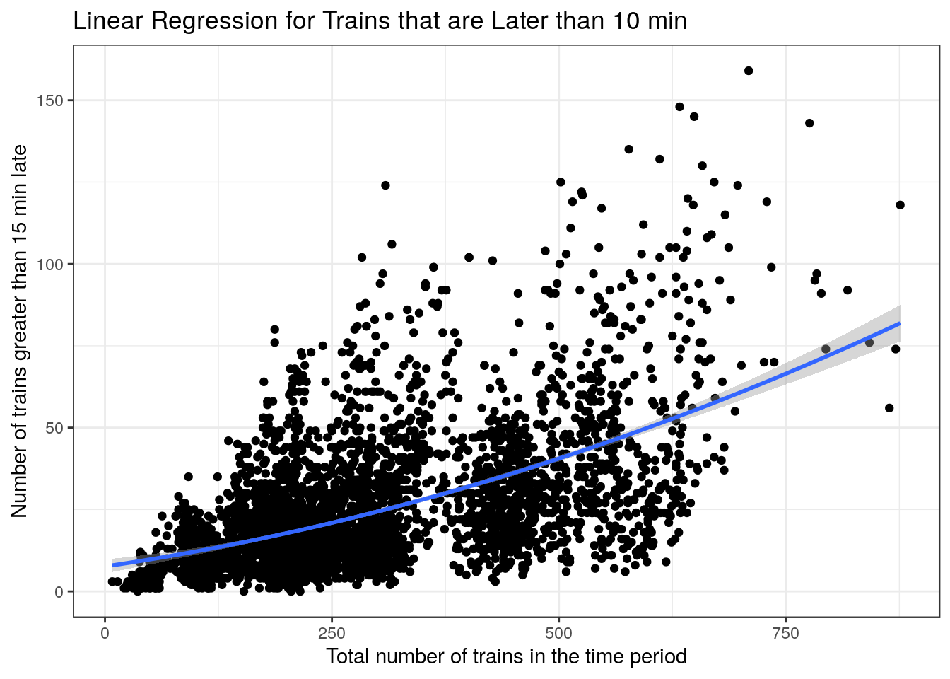
g2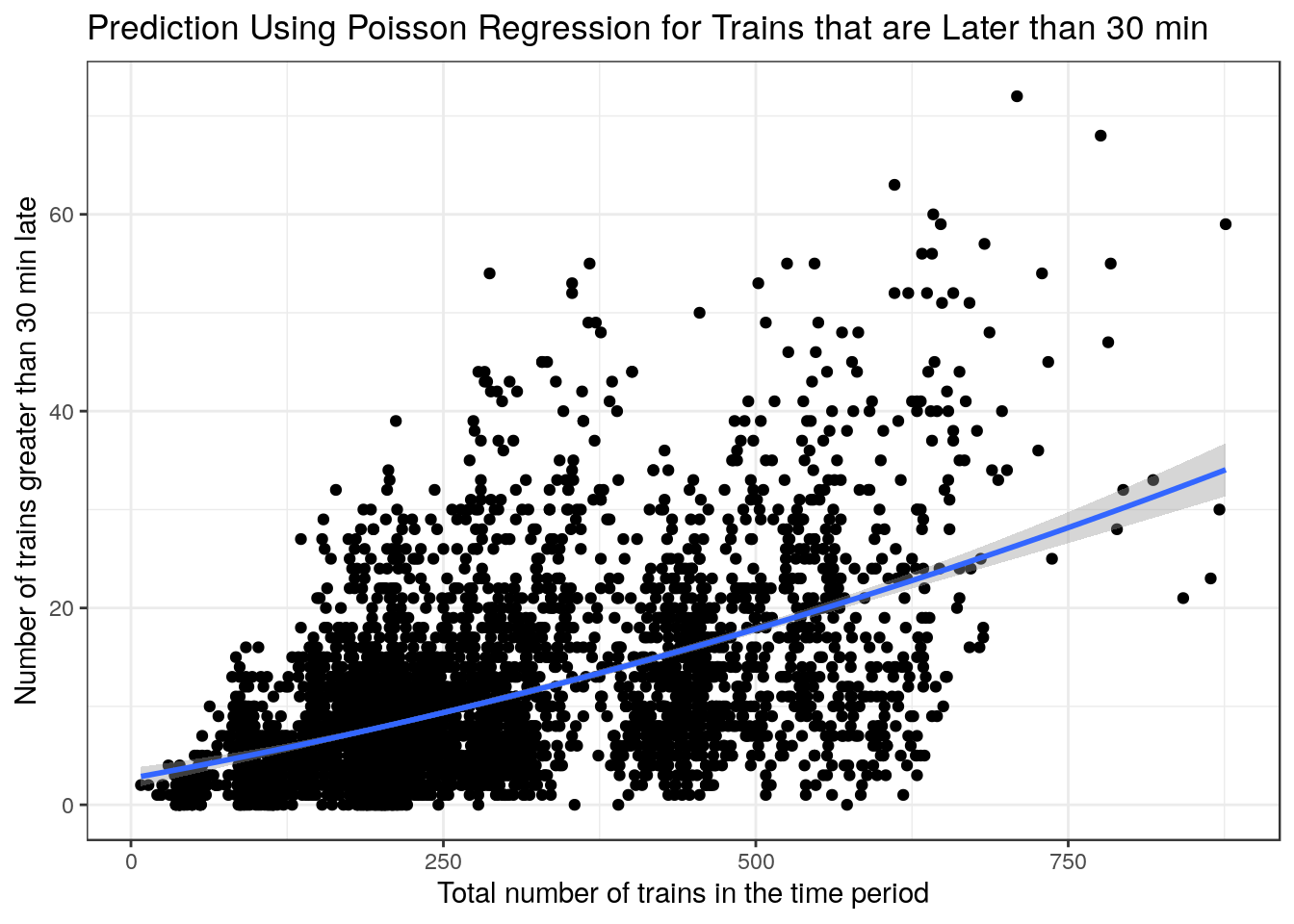
g3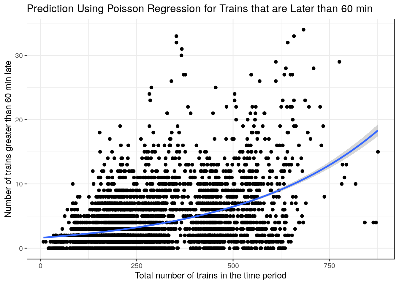
For the plots below there seems to not be the same variance relationship as the previous plots, however I still used the same models to plot the smoothers as they could give us an idea on whether if a poisson regression was a good idea or not
g1 <-
    ggplot(data = trains) + geom_point(aes(x = journey_time_avg, y = num_greater_15_min_late)) + geom_smooth(
    aes(x = journey_time_avg, y = num_greater_15_min_late),
    method = "lm",
    formula = y ~ poly(x, 2)
    ) + xlab("Total number of trains in the time period") + ylab("Number of trains greater than 15 min late") + labs(title = "Linear Regression for Trains that are Later than 10 min") + theme_bw()

    g2 <-
    ggplot(data = trains) + geom_point(aes(x = journey_time_avg, y = num_greater_30_min_late)) + geom_smooth(
    aes(x = journey_time_avg, y = num_greater_30_min_late),
    method = "lm",
    formula = y ~ poly(x, 2)
    ) + xlab("Total number of trains in the time period") + ylab("Number of trains greater than 30 min late") + labs(title = "Prediction Using Poisson Regression for Trains that are Later than 30 min") + theme_bw()

    g3 <-
    ggplot(data = trains) + geom_point(aes(x = journey_time_avg, y = num_greater_60_min_late)) + geom_smooth(
    aes(x = journey_time_avg, y = num_greater_60_min_late),
    method = stats::glm,
    formula = y ~ x ,
    method.args = list(family = poisson(link = log))
    ) + xlab("Total number of trains in the time period") + ylab("Number of trains greater than 60 min late") + labs(title = "Prediction Using Poisson Regression for Trains that are Later than 60 min") + theme_bw()

    g1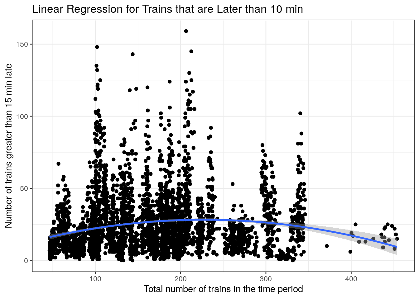
g2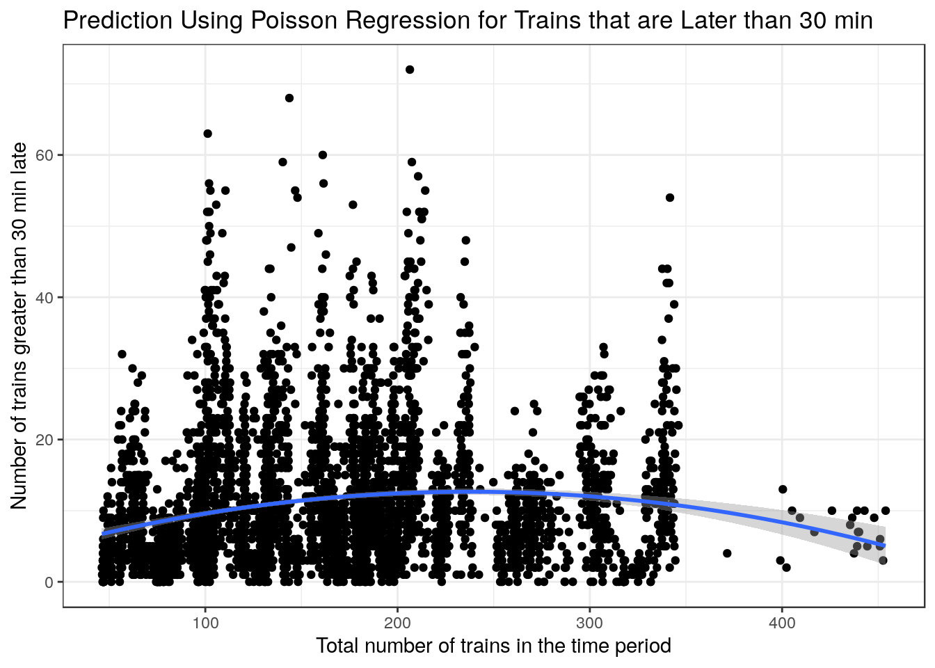
g3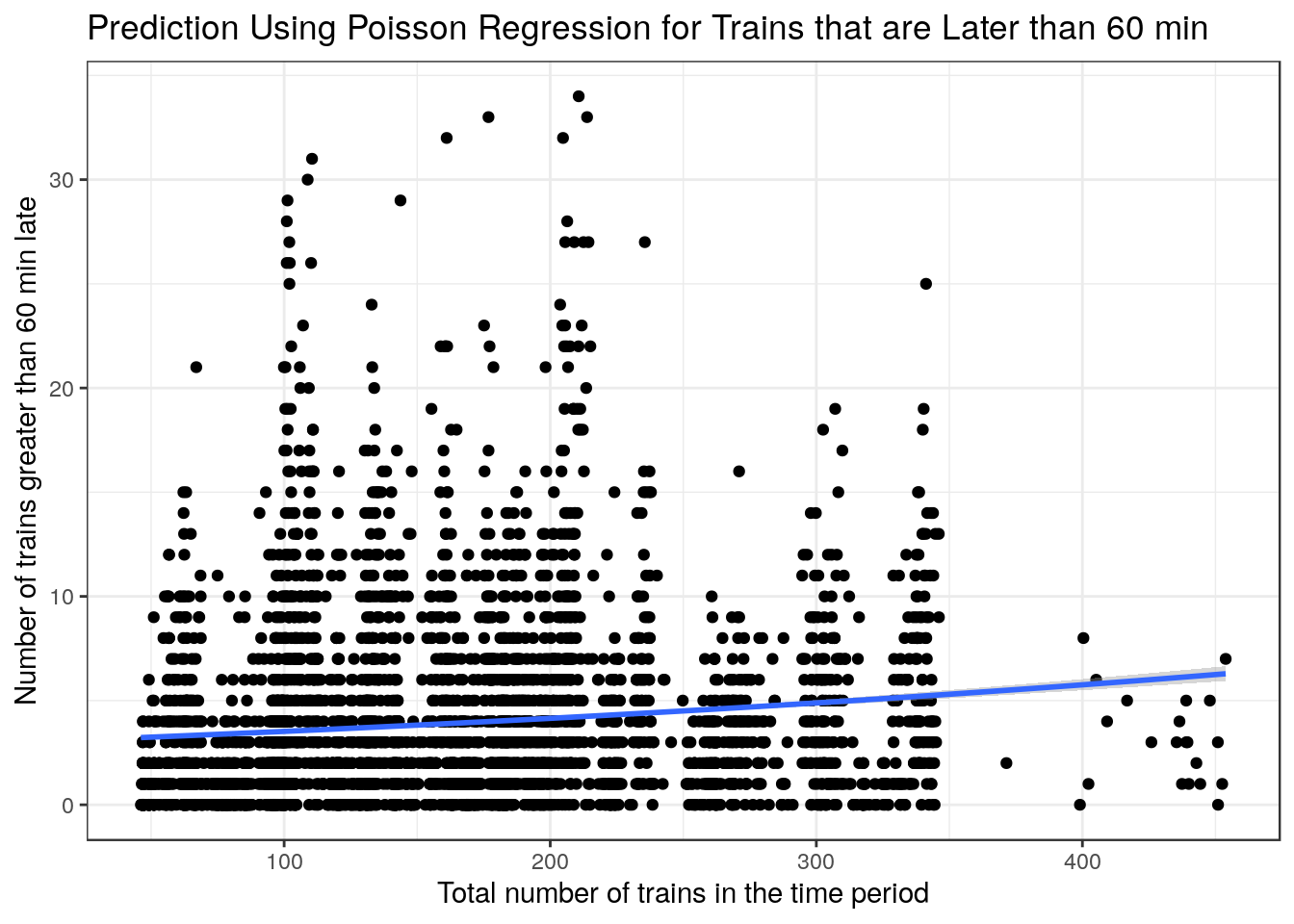
ggplot(data = trains) + geom_col(aes(x = arrival_station, y = num_greater_15_min_late)) + theme(axis.text.x = element_text(angle = 90, hjust = 1)) + xlab("City") + ylab("Trains greater than 15 min late")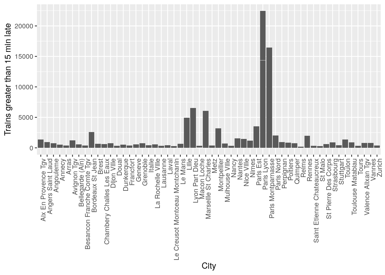
ggplot(data = trains) + geom_col(aes(x = arrival_station, y = num_greater_30_min_late)) + theme(axis.text.x = element_text(angle = 90, hjust = 1)) + xlab("City") + ylab("Trains greater than 30 min late")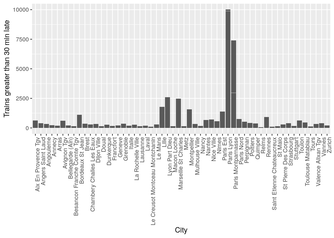
ggplot(data = trains) + geom_col(aes(x = arrival_station, y = num_greater_60_min_late)) + theme(axis.text.x = element_text(angle = 90, hjust = 1)) + xlab("City") + ylab("Trains greater than 60 min late")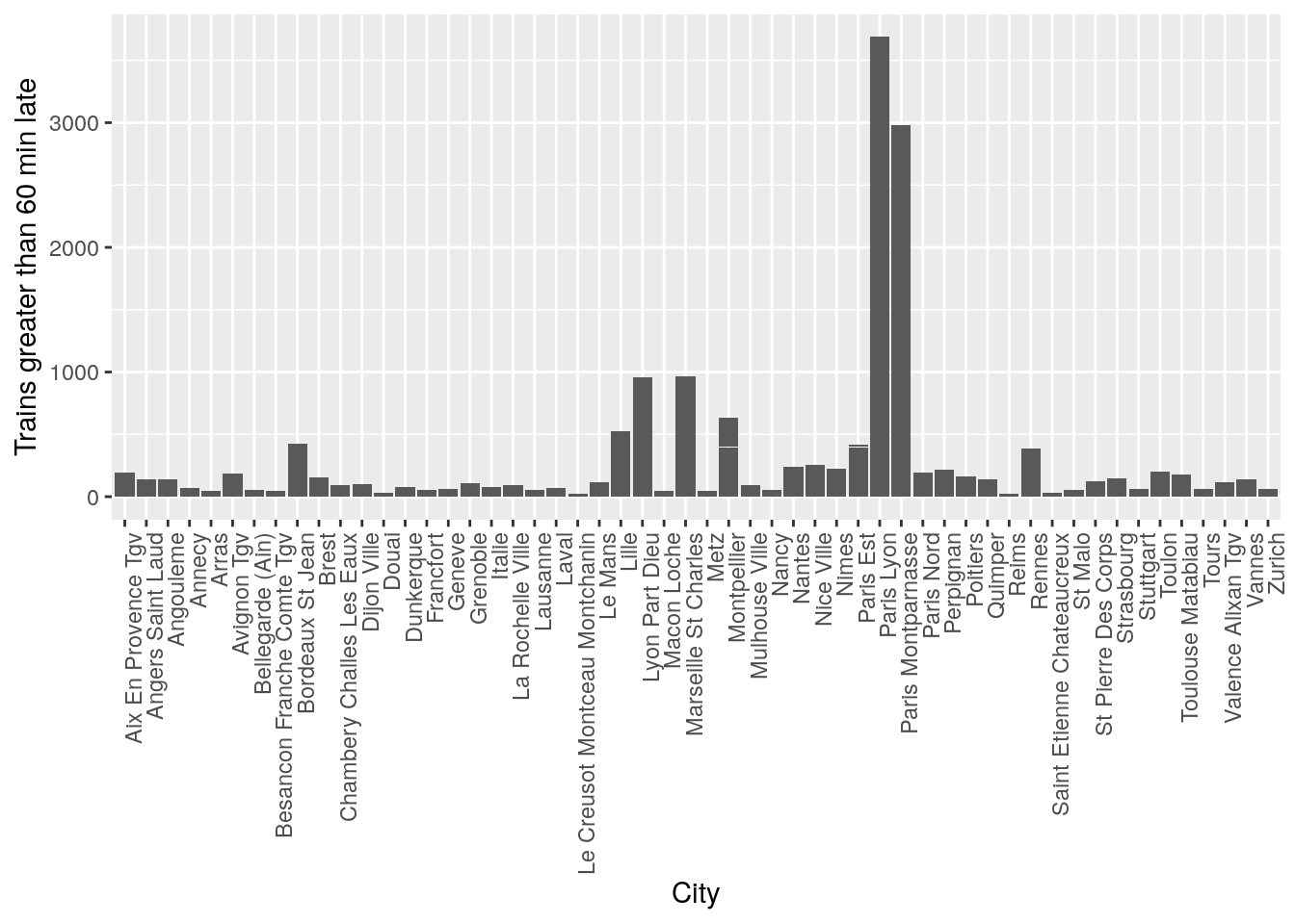
It seems like there is a pattern that certain cities have significantly more trains that are late. However this might be also due to the number of trains present in the station at that time, so when doing statistical tests, it will be important to control for variations in the total number of trains to prove that some cities are statistically more likely to have late trains.
ggplot(data = trains, aes(x = month, y = num_greater_60_min_late, fill = month)) +
       stat_summary(fun.y = sum, geom="bar", size = 1) + theme(axis.text.x = element_text(angle = 90, hjust = 1)) + xlab("Month of the Year") + ylab("Trains greater than 60 min late")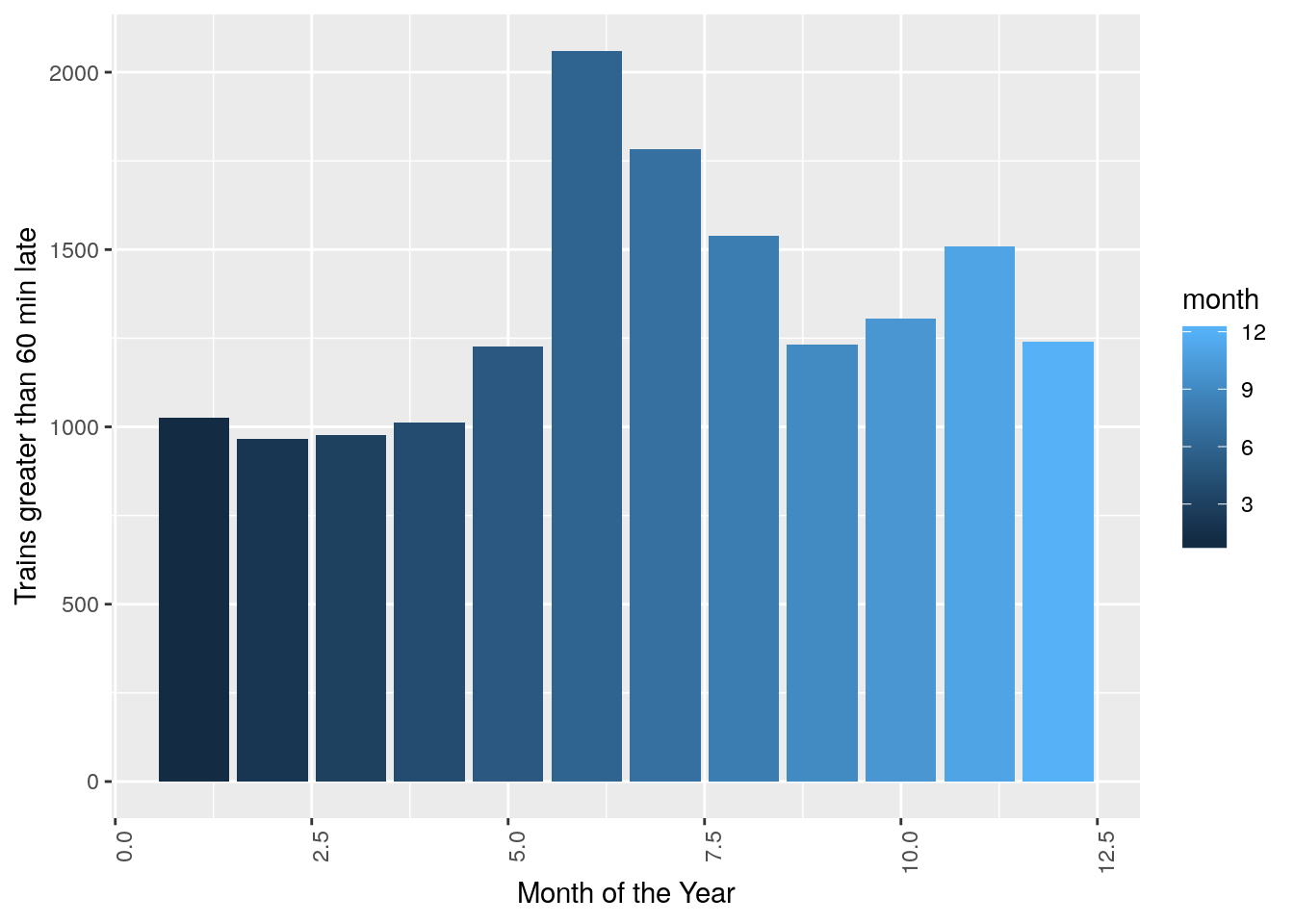
#Statistical Model and Analysis
Models
Below are the models that I built to predict the number of trains late by at least 15 mins, 30 mins and 60 mins.
train <- trains[1:nrow(trains)*0.8,]
test <- trains[nrow(trains)*0.8:nrow(trains),]


#Predict number that is later than 15min
model <- lm(data = train, num_greater_15_min_late ~ factor(departure_station)+factor(arrival_station)+ month + year + journey_time_avg + total_num_trips)

e <- residuals(model)

sHat <- predict(lm(abs(e) ~ factor(departure_station)+factor(arrival_station)+ month + year + journey_time_avg + total_num_trips , data = train))

WLS <-lm(num_greater_15_min_late ~ factor(departure_station)+factor(arrival_station)+ month + year + journey_time_avg + total_num_trips , data = train, weights = 1/(sHat^2))
#
# pander(summary.lm(WLS)["call"])
# pander(summary(WLS))
autoplot(WLS) + theme_bw()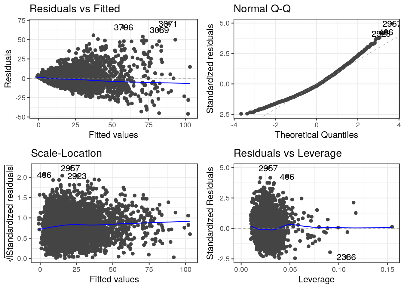
#Predict number that is later than 30min
pois.model.30 <-  glm(data = train, num_greater_30_min_late ~  total_num_trips + month + year + journey_time_avg  + factor(departure_station)+factor(arrival_station),family=poisson(link=log))

# pander(summary.lm(pois.model.30)["call"])
# pander(summary(pois.model.30))
autoplot(pois.model.30) + theme_bw()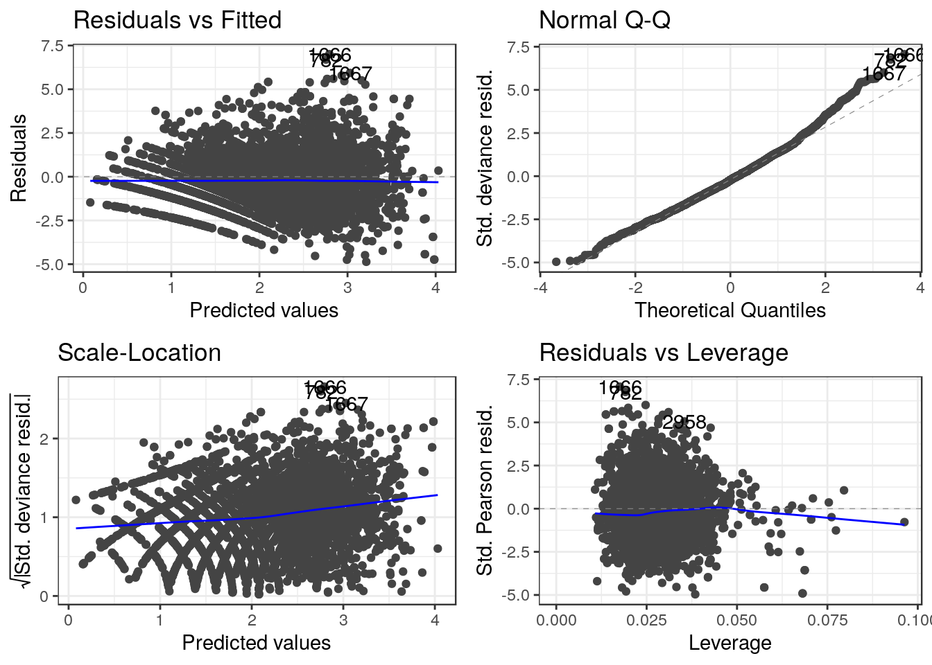
#predict number that is later than 60 min
pois.model.60 <-  glm(data = train, num_greater_60_min_late ~ factor(departure_station)+factor(arrival_station)+ month + year + journey_time_avg + total_num_trips,family=poisson(link=log))

# pander(summary.lm(pois.model.60)["call"])
# pander(summary(pois.model.60))
autoplot(pois.model.60) + theme_bw()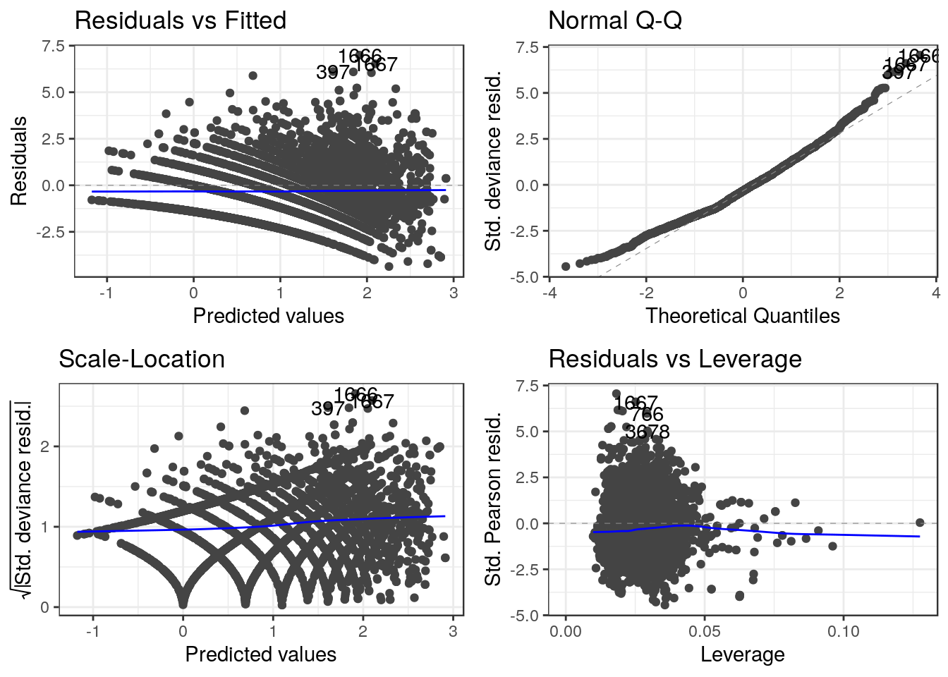
Analysis
As we said before the increase in the number of late trains in certain cities might be due to the higher number of trains in those stations. Hence, I would like to look at the anova tables when controlling for all other variables.
model <- lm(data = train, num_greater_15_min_late ~ total_num_trips + journey_time_avg + month + year + factor(departure_station) + factor(arrival_station) )

e <- residuals(model)

sHat <- predict(lm(abs(e) ~ total_num_trips + journey_time_avg + month + year + factor(departure_station) + factor(arrival_station) , data = train))

control <-lm(num_greater_15_min_late ~ total_num_trips + journey_time_avg + month + year + factor(departure_station) + factor(arrival_station) , data = train, weights = 1/(sHat^2))

pander(anova(control))| Df | Sum Sq | Mean Sq | F value | Pr(>F) | |
|---|---|---|---|---|---|
| total_num_trips | 1 | 5887 | 5887 | 3803 | 0 |
| journey_time_avg | 1 | 2760 | 2760 | 1783 | 1.828e-321 |
| month | 1 | 330 | 330 | 213.2 | 4.664e-47 |
| year | 1 | 856.4 | 856.4 | 553.2 | 1.547e-114 |
| factor(departure_station) | 53 | 2690 | 50.76 | 32.79 | 5.669e-268 |
| factor(arrival_station) | 53 | 1797 | 33.91 | 21.91 | 1.018e-179 |
| Residuals | 3915 | 6060 | 1.548 | NA | NA |
My initial guess was that the total number of trains in the station was the reason why trains were late but even after controlling for all other variations, the departure and arrival station of the trains still have a high statistical impact on the number of trains late.
Since the models for the 30 and 60 min late trains are poisson models, I cannot do an F-test controlling for other variables, but looking at how similar the data for all response variables are, I am certain that the departure and arrival stations have a significant impact on the number of late trains.
Cross-Validation Rrrors and Models’ Performances
MAE.CV <- vector(length = 10)

for (i in 1:10){
    cvTestIndex<- sample(1:nrow(trains), nrow(train)/10)
    cvDataTest  <- trains[cvTestIndex,]
    cvDataTrain <- trains[-cvTestIndex,]

        model <- lm(data = cvDataTrain, num_greater_15_min_late ~ factor(departure_station)+factor(arrival_station)+ month + year + journey_time_avg + total_num_trips)


    e <- residuals(model)

    sHat <- predict(lm(abs(e) ~ factor(departure_station) + factor(arrival_station)+ month + year + journey_time_avg + total_num_trips , data = cvDataTrain))

    weighted.ls.cv <-lm(num_greater_15_min_late ~ factor(departure_station)+factor(arrival_station)+ month + year + journey_time_avg + total_num_trips , data = cvDataTrain, weights = 1/(sHat^2))

    trainPred <- predict(weighted.ls.cv, newdata = cvDataTest)

    MAE <- sum(abs( trainPred- cvDataTest$num_greater_15_min_late))/nrow(cvDataTest)

    MAE.CV[i] <- MAE
}
MAE.CV <- mean(MAE.CV)
pander(paste("The cross valisation error for predicting trains that will be at least 15 min late is ", MAE.CV))
The cross valisation error for predicting trains that will be at least 15 min late is 7.58478418503717
MAE.CV <- vector(length = 10)

for (i in 1:10){
    cvTestIndex<- sample(1:nrow(trains), nrow(train)/10)
    cvDataTest  <- trains[cvTestIndex,]
    cvDataTrain <- trains[-cvTestIndex,]

        model <- glm(data = train, num_greater_30_min_late ~ factor(departure_station)+factor(arrival_station)+ month + year + journey_time_avg + total_num_trips,family=poisson(link=log))


    trainPred <- predict(model, newdata = cvDataTest)

    MAE <- sum((abs(trainPred- cvDataTest$num_greater_30_min_late)))/nrow(cvDataTest)

    MAE.CV[i] <- MAE
}
MAE.CV <- mean(MAE.CV)
pander(paste("The cross valisation error for predicting trains that will be at least 30 min late is ", MAE.CV))
The cross valisation error for predicting trains that will be at least 30 min late is 8.78207005307961
MAE.CV <- vector(length = 10)

for (i in 1:10){
    cvTestIndex<- sample(1:nrow(trains), nrow(train)/10)
    cvDataTest  <- trains[cvTestIndex,]
    cvDataTrain <- trains[-cvTestIndex,]

        model <- glm(data = train, num_greater_60_min_late ~ factor(departure_station)+factor(arrival_station)+ month + year + journey_time_avg + total_num_trips,family=poisson(link=log))


    trainPred <- predict(model, newdata = cvDataTest)

    MAE <- sum((abs(trainPred- cvDataTest$num_greater_60_min_late)))/nrow(cvDataTest)

    MAE.CV[i] <- MAE
}
MAE.CV <- mean(MAE.CV)
pander(paste("The cross valisation error for predicting trains that will be at least 60 min late is ", MAE.CV))
The cross valisation error for predicting trains that will be at least 60 min late is 3.16062658841709
Looking at the cross-validation errors, we can see that we can predict the number of trains late very accurately. I used a mean absolute error in order to measure the error between the true value and our predictions just to have a better idea of how close I was to the real result. Since the values for the response variables range from 0 to ~25000, this is an amazing performance. In particular, it is important to understand what the good performance of our model implies on the SNCF train delays.
Conclusion and Observations
Train delays, when not caused by external problems should be random events that are hard to predict. However since our model (which has only 6 explanatory variables) is able to predict the number of late trains. This seems to suggest that the delays in SNCF’s trains is a structural problem. In fact, looking at the anova and summary tables a few quick solutions to this delay problem seem to appear:
Increaseing the the sizes of stations or their operational capacities: The number of trains late seem to increase as the number of trains in the station increases, this seems to suggest that big train stations do not have the logistical capacity to handle the number of trains in the station.
There is an increase in the number of trains late in the summer months. This seems to suggest a lack of precautions taken by the SNCF to prevent track failures etc… due to heat.
Finally, there is a clear relationship between cities of arrival/departure and number of late trains. This relationship exists even when controling for the effect of all other variables. This suggests that the SNCF administration should investigate further certain regions in order to understand better if those regions face more infrastructure or labor issues and bring those regions closer to the national average by taking the nessecary measures.
If you have any questions or suggestions about the post, please drop me a line!