Tidy Tuesday Week 1
I will try to participate in Tidytuesday every week to practice my Tidyverse skills, so I will be posting the graphs here as well to track my experience!
I tried to use pipes as much as I can this time around, since I am trying to become more of a functional programmer! If you are curious about Tidy Tuesday check-out the github repo! Let me know if you have any questions or suggestions! Here is week 2 of 2019:
library(tidyverse)
library(gganimate)
library(patchwork)
library(ggridges)
library(lubridate)
library(viridis)
library(magrittr)
library(knitr)
library(kableExtra)

data <- read_csv("../data/Tidytuesday/IMDb_Economist_tv_ratings.csv")
summary(data) %>% kable(caption = "Fig 1: Summary of The Data") %>%
kable_styling(bootstrap_options = "hover")| titleId | seasonNumber | title | date | av_rating | share | genres | |
|---|---|---|---|---|---|---|---|
| Length:2266 | Min. : 1.000 | Length:2266 | Min. :1990-01-03 | Min. :2.704 | Min. : 0.00 | Length:2266 | |
| Class :character | 1st Qu.: 1.000 | Class :character | 1st Qu.:2007-01-22 | 1st Qu.:7.731 | 1st Qu.: 0.10 | Class :character | |
| Mode :character | Median : 2.000 | Mode :character | Median :2012-12-07 | Median :8.115 | Median : 0.32 | Mode :character | |
| NA | Mean : 3.264 | NA | Mean :2010-11-06 | Mean :8.061 | Mean : 1.28 | NA | |
| NA | 3rd Qu.: 4.000 | NA | 3rd Qu.:2016-03-08 | 3rd Qu.:8.490 | 3rd Qu.: 1.09 | NA | |
| NA | Max. :44.000 | NA | Max. :2018-10-10 | Max. :9.682 | Max. :55.65 | NA |
head(data) %>% kable(caption = "Fig 2: Extract from Data") %>%
kable_styling(bootstrap_options = "hover")| titleId | seasonNumber | title | date | av_rating | share | genres |
|---|---|---|---|---|---|---|
| tt2879552 | 1 | 11.22.63 | 2016-03-10 | 8.4890 | 0.51 | Drama,Mystery,Sci-Fi |
| tt3148266 | 1 | 12 Monkeys | 2015-02-27 | 8.3407 | 0.46 | Adventure,Drama,Mystery |
| tt3148266 | 2 | 12 Monkeys | 2016-05-30 | 8.8196 | 0.25 | Adventure,Drama,Mystery |
| tt3148266 | 3 | 12 Monkeys | 2017-05-19 | 9.0369 | 0.19 | Adventure,Drama,Mystery |
| tt3148266 | 4 | 12 Monkeys | 2018-06-26 | 9.1363 | 0.38 | Adventure,Drama,Mystery |
| tt1837492 | 1 | 13 Reasons Why | 2017-03-31 | 8.4370 | 2.38 | Drama,Mystery |
colnames(data) <- c("Id", "Season Number", "Title", "Date", "Average Rating", "Share", "Genres")
# data %>% transmute(Date = as.Date, "%y-%m-%d")
data %<>% mutate(Year = year(Date))
data %>% ggplot +
geom_density_ridges(aes(x = `Average Rating`, y = Year, group = Year, fill= Year)) +
scale_fill_viridis(name = "Tail probability", direction = -1) +
theme_bw() +
guides(fill = F) +
coord_flip() +
labs(title = "IMDB Rating Distributions Over the Years") 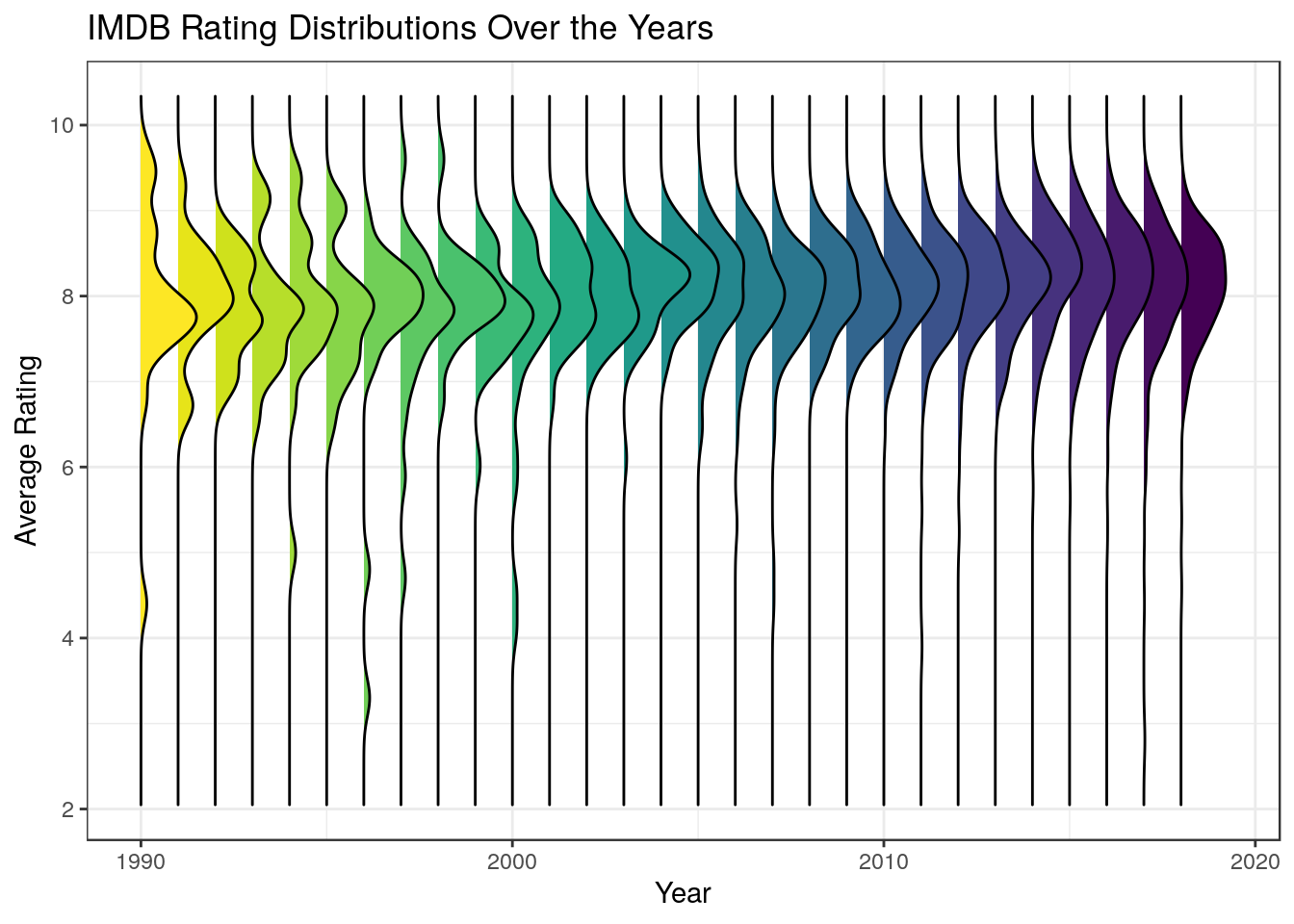
data %>% filter(Title %in%  ( data %>%  count(Title) %>% arrange(n %>% desc) %>% top_n(10,n) %>% pull(Title) )) %>% ggplot +
    geom_point(aes(x = Year, y = `Average Rating`, group = Title, color = Title)) +
    geom_smooth(aes(x = Year, y = `Average Rating`,color = Title), method = "loess",fill = NA) +
    guides(color = F) +
    labs(title = "IMDB Ratings of the 10 Longest TV Series over Time: \n{closest_state} ") +
    transition_states(states = Title, state_length = 2)  +
    ylab("Average IMDB Rating") + theme_bw()